UniformStreamlines.jl
Evenly-spaced streamlines for 2-D, 3-D, and N-D vector fields in Julia.
UniformStreamlines.jl implements the Jobard–Lefer algorithm to produce streamlines that are uniformly distributed across a domain. It works with function-defined or grid-defined velocity fields and supports Plots.jl and Makie.jl for visualization.
Installation
using Pkg
Pkg.add("UniformStreamlines")
Quick Start
using UniformStreamlines

xs = LinRange(-2, 2, 200)
ys = LinRange(-2, 2, 200)

# Separate component functions
str = evenstream(xs, ys, (x, y) -> -y, (x, y) -> 1 + x - y^2)

# Or a single vector-valued function — Tuple return = zero allocations
str = evenstream(xs, ys, x -> (-x[2], 1 + x[1] - x[2]^2))
Plot with Plots.jl:
using Plots
streamlines(str)
Or with Makie:
using CairoMakie
streamlines(str)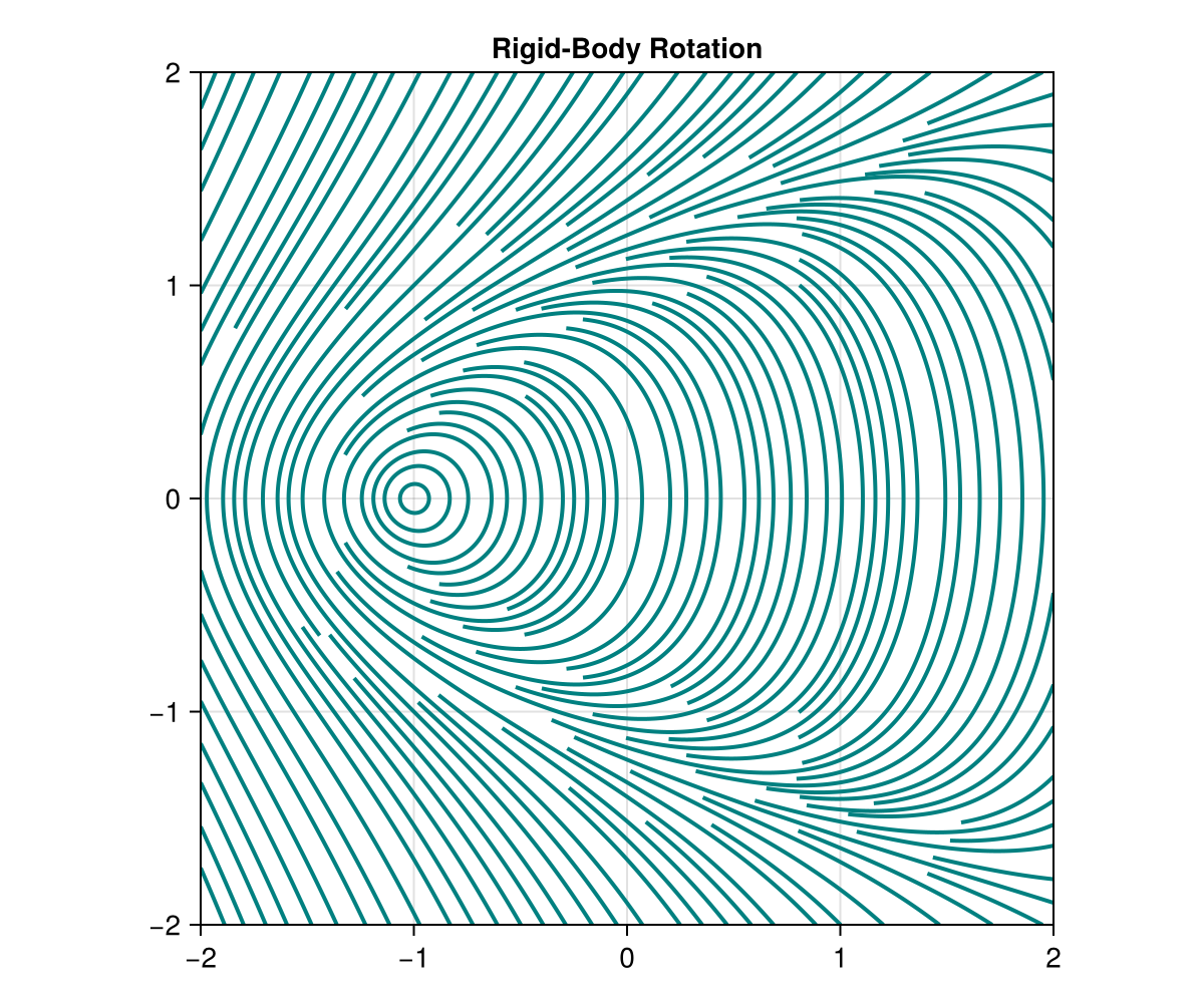
Features
Field Input Styles
evenstream accepts four styles of velocity field input:
xs = LinRange(-2, 2, 100);  ys = LinRange(-2, 2, 100)

# 1. Separate component functions — scalar coordinates, zero allocations
str = evenstream(xs, ys, (x, y) -> -y, (x, y) -> x)

# 2. Single vector-valued function — receives p::SVector, return a Tuple or SVector
str = evenstream(xs, ys, p -> (p[2], -p[1]))

# 3. Varargs function — receives scalar coordinates, auto-detected
f(x, y) = (sin(x), cos(y))
str = evenstream(xs, ys, f)

# 4. Callable struct — useful when the field carries shared state
struct RotField; α::Float64 end
(F::RotField)(p) = (p[2] * F.α, -p[1])
str = evenstream(xs, ys, RotField(1.5))

# 5. Pre-computed arrays — linearly interpolated at integration points
U = [-y for x in xs, y in ys];  V = [x for x in xs, y in ys]
str = evenstream(xs, ys, U, V)For simple functions Julia can inline and eliminate all allocations regardless of return type. For named or @noinline functions, returning a Vector allocates once per field evaluation. Since the field is called millions of times during integration, this compounds: in benchmarks, Vector-returning functions produce ~20,000× more allocations than Tuple- or SVector-returning equivalents. Prefer Tuple or SVector returns when writing named field functions.
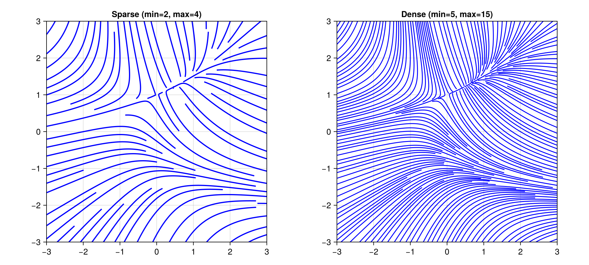
Density Control
Adjust min_density and max_density to control how tightly streamlines are packed:
xs = LinRange(-3, 3, 200)
ys = LinRange(-3, 3, 200)

# Sparse
str_sparse = evenstream(xs, ys, (x, y) -> -1 - x^2 + y, (x, y) -> 1 + x - y^2;
                    min_density=2, max_density=4)

# Dense
str_dense = evenstream(xs, ys, (x, y) -> -1 - x^2 + y, (x, y) -> 1 + x - y^2;
                   min_density=5, max_density=15)
Both parameters are unitless multipliers that scale an internal base grid of 10 cells per axis:
min_density(default4) — Controls the seeding grid. The domain is divided into10 × min_densitycells per axis. One candidate seed point is placed per cell, so a higher value means more candidate starting points and denser coverage.max_density(default10) — Controls the collision-detection grid. The domain is divided into10 × max_densitycells per axis. When a streamline is being integrated, it checks this finer grid to decide whether it is too close to an existing streamline. A higher value allows streamlines to pass closer together before being truncated.
The ratio max_density / min_density determines how much room there is between the minimum spacing (set by the collision grid) and the seeding spacing. Typical values:
| Style | min_density | max_density |
|---|---|---|
| Sparse | 2 | 4 |
| Normal | 4 (default) | 10 (default) |
| Dense | 5–8 | 15–30 |
Coloring
colorize(str, f) computes a per-point value for each vertex in the streamlines. f receives the position p and velocity v at that point.
Scalar coloring — f returns a Real, pair the result with a colormap:
str = evenstream(xs, ys, (x, y) -> sin(π*x) * cos(π*y), (x, y) -> 0.2y)

c = colorize(str, :norm)                              # speed (built-in shortcut)
c = colorize(str, (p, v) -> p[1]^2 + p[2]^2)         # distance² from origin
c = colorize(str, (p, v) -> v[1] / norm(v))           # cos(angle) with x-axis

streamlines!(ax, str; color=c, colormap=:viridis)
Built-in scalar symbols: :norm / :speed, :vx / :u, :vy / :v, :vz / :w, :x, :y, :z.
Direct color — f returns a Colorant, used as-is without a colormap:
using Makie: RGBAf

c = colorize(str, (p, v) -> RGBAf(v[1], v[2], 0, 1))   # color by velocity direction

streamlines!(ax, str; color=c)
With Plots.jl, pass a scalar color array via line_z:
using Plots
streamlines(str; line_z=c, color=:viridis)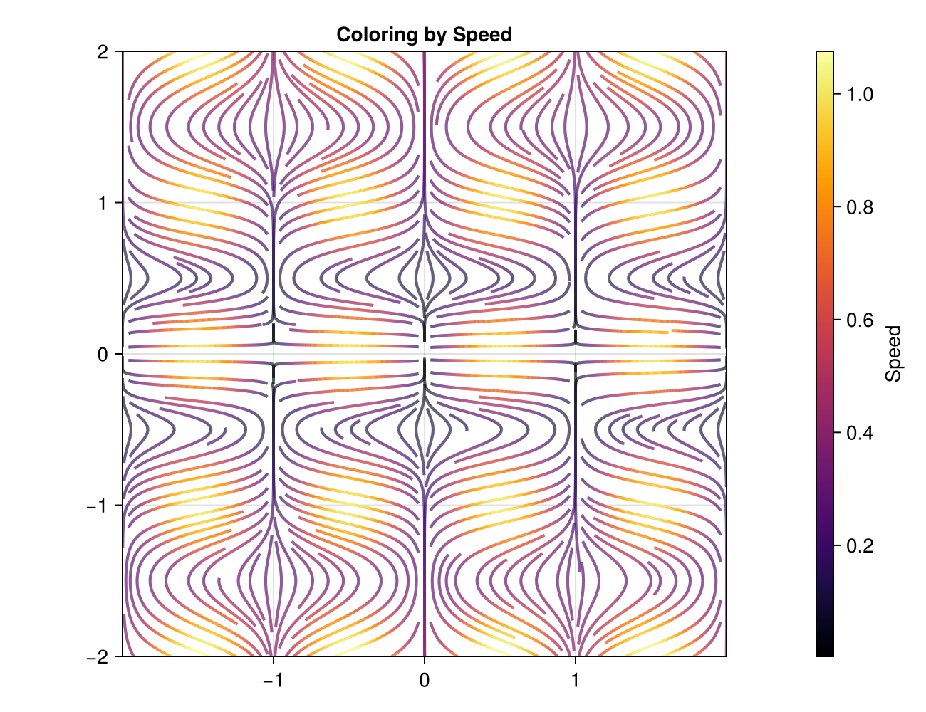
Arrows
Add directional arrows along streamlines with with_arrows=true. Arrows are placed uniformly along the arc length of each streamline by default, so spacing is consistent regardless of how densely the path is sampled:
# Makie — uniform arrows with automatic spacing
streamlines(str; with_arrows=true)

# Plots.jl
streamlines(str; with_arrows=true)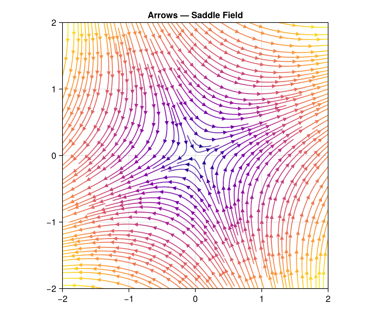
You can control the arc-length distance between arrows with arrows_spacing:
# Tighter arrow spacing
streamlines(str; with_arrows=true, arrows_spacing=0.15)

# Wider arrow spacing
streamlines(str; with_arrows=true, arrows_spacing=0.5)
Alternatively, use arrows_every to place an arrow every N-th path vertex. This is faster but produces non-uniform spacing when vertex density varies:
# Vertex-based placement (non-uniform)
streamlines(str; with_arrows=true, arrows_every=20)
Control arrow size with markersize:
# Makie
streamlines(str; with_arrows=true, markersize=8)   # small
streamlines(str; with_arrows=true, markersize=20)  # large

# Plots.jl
streamlines(str; with_arrows=true, markersize=0.5)  # half size
streamlines(str; with_arrows=true, markersize=2.0) # double size![]()
NaN Masking
Return NaN from velocity functions to mask out regions of the domain. Streamlines will not enter or cross masked areas:
u(x, y) = (x+1)^2 + y^2 < 1 ? NaN : x + y
v(x, y) = (x+1)^2 + y^2 < 1 ? NaN : x - y

str = evenstream(xs, ys, u, v)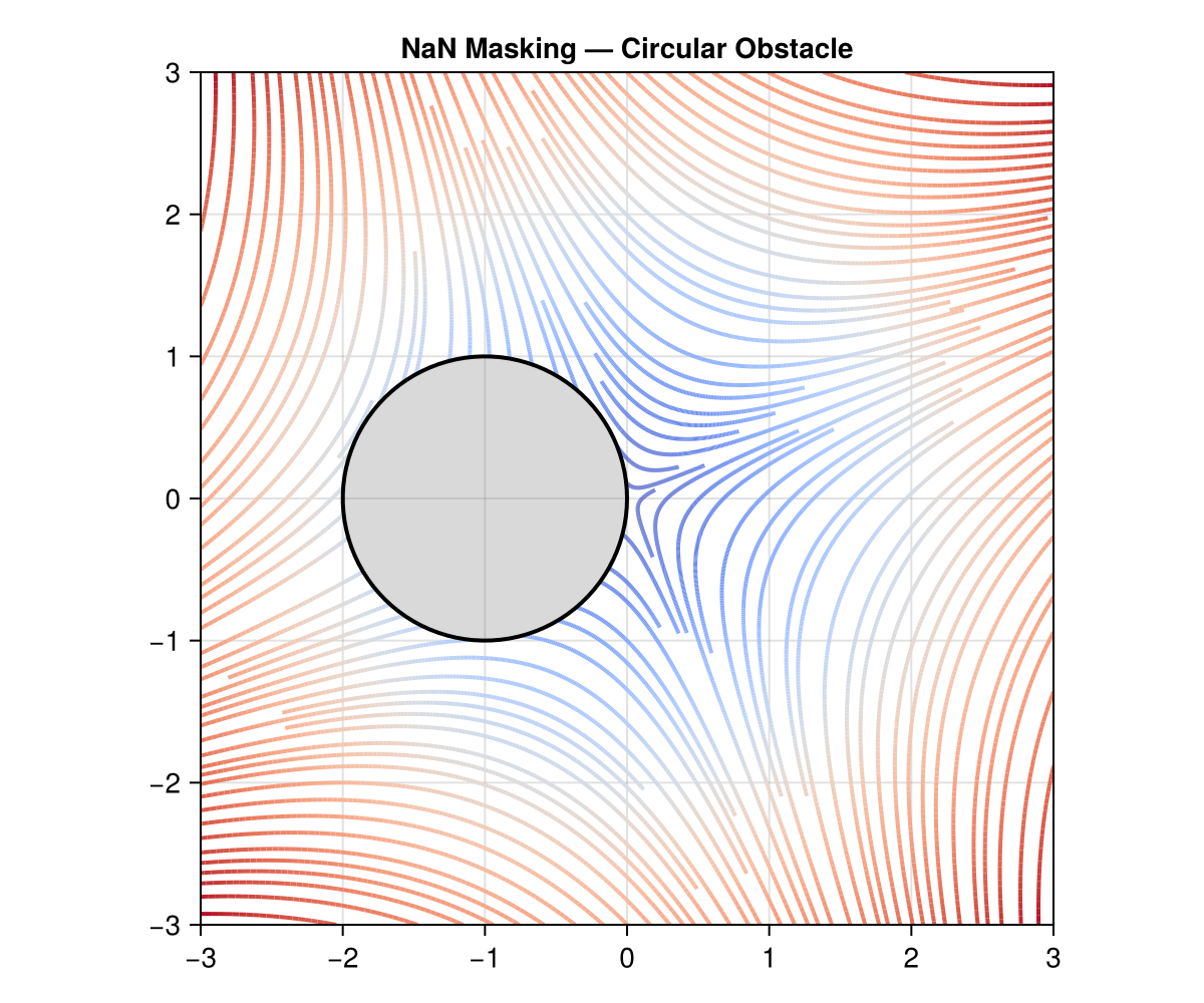
Seed Points
Provide explicit seed points to control where streamlines originate. Two equivalent formats are accepted:
# Pair of N-vectors, one per axis
seed_x = [-1.0, 0.0, 1.0]
seed_y = [ 0.0, 0.0, 0.0]
str = evenstream(xs, ys, (x, y) -> x + y, (x, y) -> x - y; seeds=(seed_x, seed_y))

# Tuple of D-vectors, one per seed point
seeds = ([-1.0, 0.0], [0.0, 0.0], [1.0, 0.0])
str = evenstream(xs, ys, (x, y) -> x + y, (x, y) -> x - y; seeds=seeds)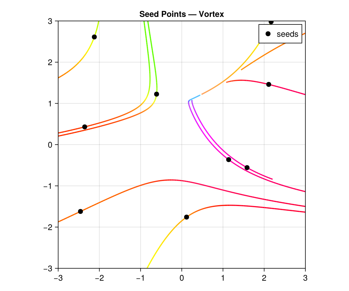
Unbroken Streamlines
By default, streamlines are truncated when they approach an existing streamline. Set allow_collisions=true to let them pass through each other:
str = evenstream(xs, ys, (x, y) -> -y / (x^2 + y^2 + 0.1),
                     (x, y) ->  x / (x^2 + y^2 + 0.1);
             allow_collisions=true)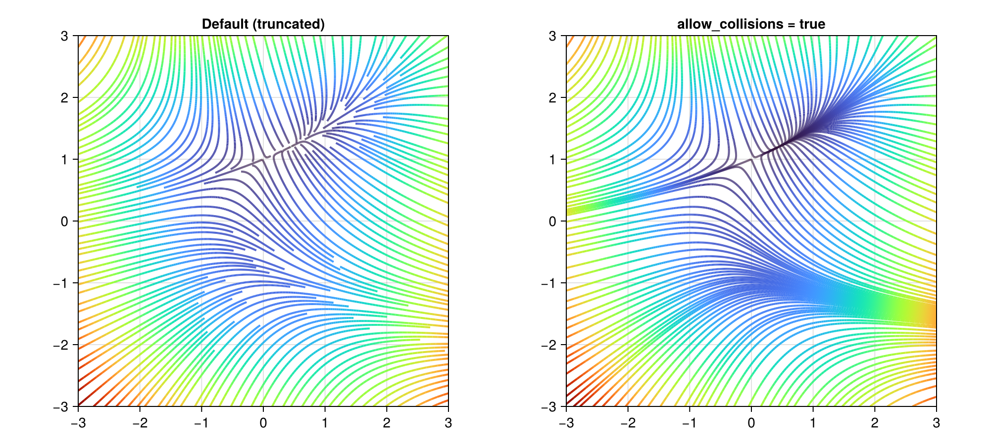
3-D Streamlines
The same interface extends to three dimensions:
xs = LinRange(-2, 2, 50)
ys = LinRange(-2, 2, 50)
zs = LinRange(-2, 2, 50)

str3 = evenstream(xs, ys, zs,
              (x, y, z) -> -y,
              (x, y, z) ->  x,
              (x, y, z) ->  0.3z)
A more interesting example — the Arnold–Beltrami–Childress (ABC) flow with directional arrows:
A, B, C = 1.0, √2, √3
str3 = evenstream(xs, ys, zs,
              (x, y, z) -> A * sin(z) + C * cos(y),
              (x, y, z) -> B * sin(x) + A * cos(z),
              (x, y, z) -> C * sin(y) + B * cos(x);
              min_density=2, max_density=4)
c3 = colorize(str3, :norm)

using GLMakie
streamlines(str3; color=c3, colormap=:magma,
            with_arrows=true, markersize=0.12)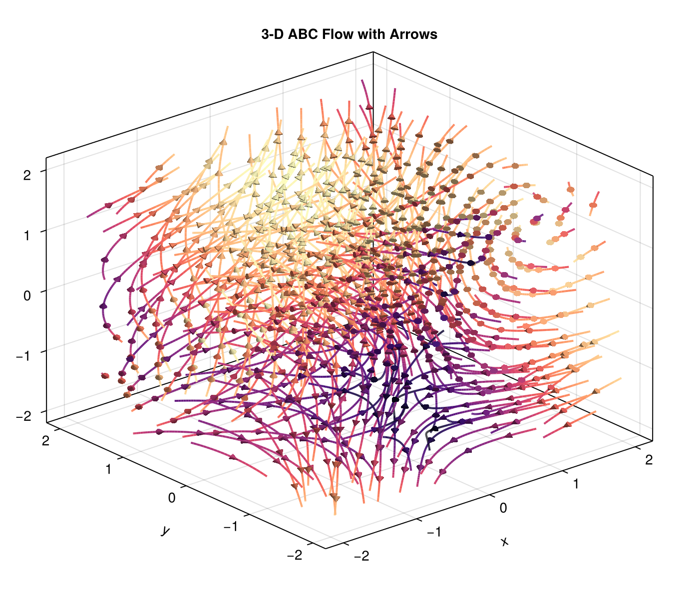
N-D Streamlines
For arbitrary dimensions, use the tuple form:
axs = (LinRange(-2, 2, 50), LinRange(-2, 2, 50), LinRange(-2, 2, 50), LinRange(-2, 2, 50))
fns = ((x, y, z, t) -> -y, (x, y, z, t) -> x, (x, y, z, t) -> z, (x, y, z, t) -> -t)
str4 = evenstream(axs, fns)
Calling Conventions
evenstream supports two equivalent calling styles:
Flat form — pass axes and velocity components as separate positional arguments. This is the most convenient syntax for 2-D and 3-D fields:
# 2-D with functions
str = evenstream(xs, ys, (x, y) -> -y, (x, y) -> x)

# 2-D with matrices
str = evenstream(xs, ys, U, V)

# 3-D with functions
str = evenstream(xs, ys, zs, (x,y,z) -> -y, (x,y,z) -> x, (x,y,z) -> 0.3z)

# 3-D with matrices
str = evenstream(xs, ys, zs, U, V, W)
Tuple form — pass axes as a tuple and velocity components as a tuple. This is the general N-D interface, but works in any dimension:
# 2-D (tuple form)
str = evenstream((xs, ys), ((x,y) -> -y, (x,y) -> x))

# 3-D (tuple form)
str = evenstream((xs, ys, zs), ((x,y,z) -> -y, (x,y,z) -> x, (x,y,z) -> 0.3z))

# 4-D
str = evenstream((xs, ys, zs, ts), (f1, f2, f3, f4))

# With pre-computed arrays
str = evenstream((xs, ys), (U, V))
Both forms accept the same keyword arguments (min_density, max_density, seeds, allow_collisions, etc.). The flat form is simply a convenience wrapper that forwards to the tuple form internally.
API Summary
| Function | Description |
|---|---|
evenstream | Compute evenly-spaced streamlines |
colorize | Compute per-point scalar or color values |
streamarrows | Extract arrow glyphs for visualization |
streamlines / streamlines! | Plot recipe (Plots.jl or Makie) |
Keyword arguments to evenstream
| Keyword | Default | Description |
|---|---|---|
min_density | 4 | Seeding grid density (10 × min_density cells/axis). Higher → more seed candidates → denser coverage. |
max_density | 10 | Collision grid density (10 × max_density cells/axis). Higher → streamlines may pass closer together. |
seeds | nothing | Explicit seed points — tuple of D-vectors (one per point) or pair of N-vectors (one per axis) |
min_length | 2 | Discard streamlines with fewer than this many vertices |
allow_collisions | false | Allow streamlines to cross each other |
stepsize | adaptive | Arc-length step size (physical distance per integration step). Velocity is normalized internally, so this controls spatial resolution independent of field magnitude. Default: min(norm(domain) / (10 × max_density × 10), 0.05) |
Keyword arguments for Plots.jl recipe
| Keyword | Default | Description |
|---|---|---|
with_arrows | false | Show directional arrowheads |
arrows_spacing | automatic | Arc-length spacing between arrows (uniform placement) |
arrows_every | nothing | Legacy: place an arrow every N vertices; overrides arrows_spacing |
markersize | 1.0 | Scale factor for arrow size |
line_z | — | Per-point color values from colorize |
Keyword arguments for Makie recipe
| Keyword | Default | Description |
|---|---|---|
with_arrows | false | Show directional arrowheads |
arrows_spacing | automatic | Arc-length spacing between arrows (uniform placement) |
arrows_every | nothing | Legacy: place an arrow every N vertices; overrides arrows_spacing |
markersize | 12 (2-D) / 0.08 (3-D) | Size of arrowhead markers |
color | :blue | Line / arrowhead color or per-point vector from colorize |
linewidth | inherited | Width of streamlines |
colormap | — | Colormap for color-mapped data |